

Computer Vision's Giant Leaps
Computer Vision's Giant Leaps
From feline cortices to self-driving cars

There are a million how-to’s introducing convolutional neural networks, their high-level principles, and their implementation. (In my opinion, the best introductions can be found here, here, and here.)
But where did they come from? Let’s run through a few of the boldest steps computer vision took from its inspiration in feline cortices to its application in self-driving cars. These ideas might be older than you think!
Today’s Stepping Stones:
Hubel, Weisel and the Visual Cortex (1959)
The Mighty Neurocognitron (1980)
LeCun Backprops through Object Recognition (1999)
AlexNet vs. ImageNet (2012)
DeepLab’s Dilations, Etc. (2016)
Capsule Networks (2017)
Transformers?? For images??? (2020)
1959: Hubel and Wiesel’s Cat Cortices
Computer vision arguably began in 1959, with a revolution in our understanding of the visual cortex—the region of the brain where humans process and interpret what they see.
Biologists Hubel and Wiesel showed that the visual cortex is hierarchal: groups of neurons look for specific features in small neighborhoods of the retina—for example, different kinds of edges—and pool their findings together before passing them along to higher-level groups, which look for further “zoomed-out” or abstracted features.
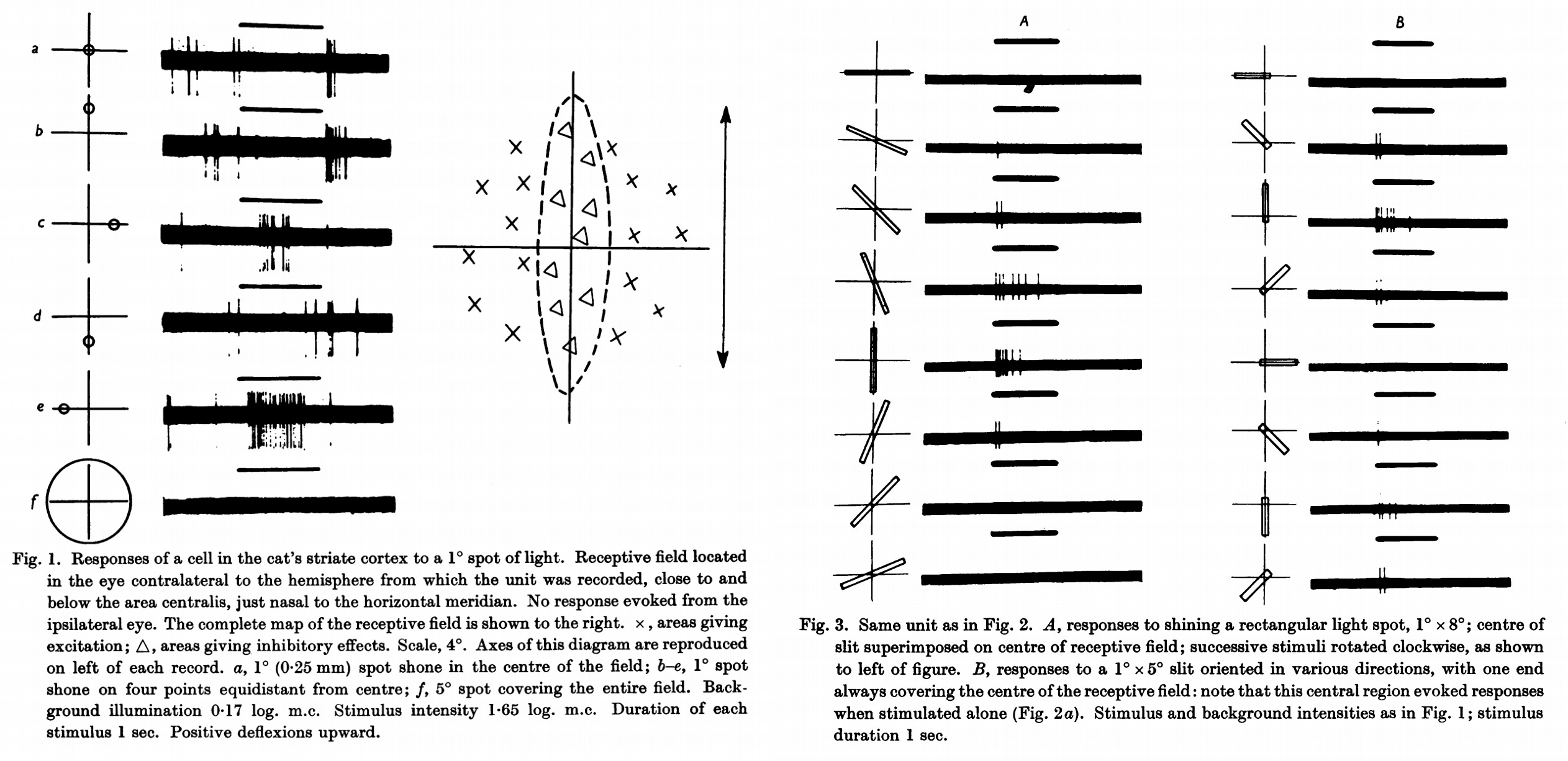
They showed, in short, that vision is achieved by a hierarchy of local computational units, looking for specific thing—in their words, “a specificity of stimuli, in shape, size and orientation”) in specific places (what they termed “receptive fields”).
Convolutional neural networks (CNNs) were proposed to model these characteristics of human vision. To mimic neuron groups in the visual cortex, they employ a unit of computation—convolutions—that learn, during training, to identify important features in a small “receptive field” of their input. This process repeats in layers: individual convolutions produce (activation) “maps” of where they think their feature roughly exists in a given input; these maps are reduced in size (think of shrinking the dimensions of an image) and become the input for another layer of convolutions, which look for more abstract things.
To acquaint yourself with convolutional arithmetic, I recommend this page. I’ll review just a few key pieces of vocab.
A feature volume is the intermediate representation of data in a convolutional neural network, with height, width, and channel dimensions (hence “volume”—this excludes batching). Each convolution applied to a feature volume creates a new feature volume with different dimensions, depending on the convolution’s hyperparameters.
There are two ways that classification networks commonly reduce the dimensionality of the feature volume: pooling and convolutional stride.
Max pooling (which didn’t show up until 1993) does what the name implies, replacing a neighborhood of pixel values with the local maximum:

There’s also average pooling, which replaces with the local average.
A convolution’s stride is simply a measure of how much the kernel travels each step when “sliding over” the feature volume. Loosely, a larger stride means the kernel will take fewer steps before reaching the “end” (along one dimension), meaning it will compute fewer activations, yielding a smaller output volume.
For example, with appropriate padding, a convolutional stride of 2 will halve the height and width of an input feature volume.
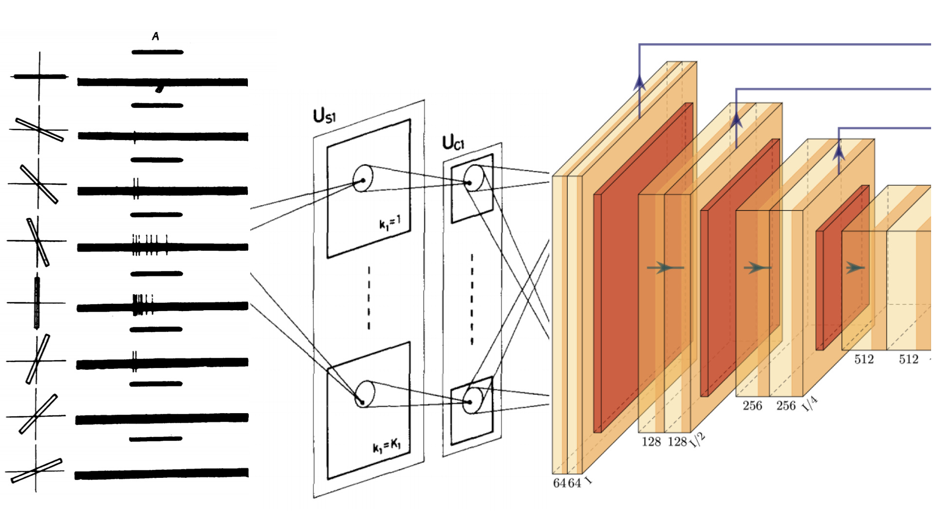
1980: Fukushima’s Neurocognitron
In the paper where CNNs (of a sort) were first proposed, Fukushima, a Japanese scientist, cites the work of Hubel and Wiesel as inspiration, noting that
The structure of this network has been suggested by that of the visual nervous system of the vertebrate…and acquires an ability to recognize stimulus patterns based on the geometrical similarity of their shapes, without being affected by their position nor by small distortions (193).
Fukushima noted that the local attention and continual pooling-down of convolutional neural networks enabled them to handle a wide array of slight changes in their vision, to be more robust—one could say, more “human”.

But Fukushima’s CNNs were still missing something: the ideal training algorithm. When Fukushima trained CNNs, he simply presented them with many images and changed their convolutional features based on a few heuristic criteria. What he called “learning without a teacher” is now called “unsupervised learning”: giving the machine no human-labeled information about the data. The way machines learn is still far simpler than how humans do it, but great strides have been made since the 1980’s, chiefly through the introduction of supervised learning and, relatedly, backpropagation.
1999: LeCun Uses Backprop for Object Recognition
The 90’s saw the advent of backpropagation, gradient-based learning, and supervised learning, which makes use of human data labels. Together, these ideas would form the foundation of modern deep learning, by making it much quicker (and often easier) to train neural networks.
When LeCun and company trained a CNN using gradient-based learning with backprop, they challenged it to classify handwritten digits from zero to nine. For each image, the network would learn convolutional features to make a prediction about which number it was seeing. This is called the forward pass.
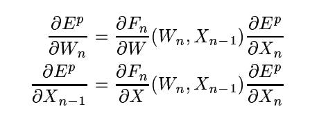
The backward pass would begin when the network received a label: the correct answer. It would compute a loss function—some measure of how wrong it was—and then calculate, using calculus, how each of convolution at every layer led it to being wrong. Backpropagation (or “Backprop”) gets its name because the gradients at the end of the model propagate (via the chain rule) back through the network to the input, providing a signal at every layer for how best to tweak parameters.
The key consequence of backprop is that any fully differentiable model can be trained via gradient descent, in place of inferior search methods.
By shuffling its convolutions “away” from that wrongness, over many images, LeCun’s network (“LeNet”) learned proper classifications, along with the features necessary to make them consistently.
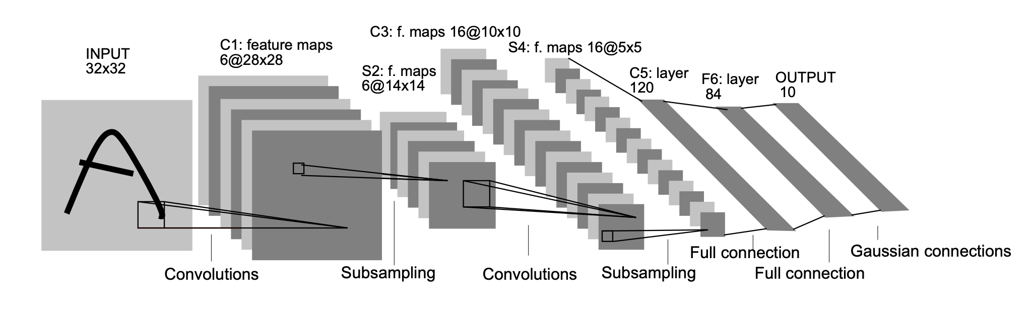
LeCun remarks that
Since all the weights are learned with back-propagation, convolutional networks can be seen as synthesizing their own feature extractors, and tuning them to the task at hand (6).
And it’s here, perhaps, that LeCun and his coauthors earned their reputations as godparents of deep learning, when they performed the automatic feature-extraction central to the field: they observed (emphasis added)
it is possible, and even advantageous, to feed the system directly with minimally processed images and to rely on learning to extract the right set of features (319).
In other words: why spend our time creating human-written rules, when we can train systems to come up with better, more effective ones from nothing more than a dataset with labels? This is the intuition that led to superhuman radiology and self-driving cars that crash less often than we do.
2012: AlexNet Crushes the Competition
AlexNet put the “deep” in deep computer vision, leveraging the power of GPUs to build deeper CNNs and achieve higher accuracies. It wasn’t the first to do this, but it was the most influential, with upwards of 75k citations (at time of writing).
As you can see below, AlexNet is bigger than LeNet in all dimensions. Its input images (from the 1000-class ImageNet dataset—which deserves its own history—versus the simpler 10-class MNIST digits) were much larger; it featured far more layers; and each layer had far more feature maps / channels. Not to mention more fully-connected layers, all of them with over 10x the number of neurons in LeNet’s!
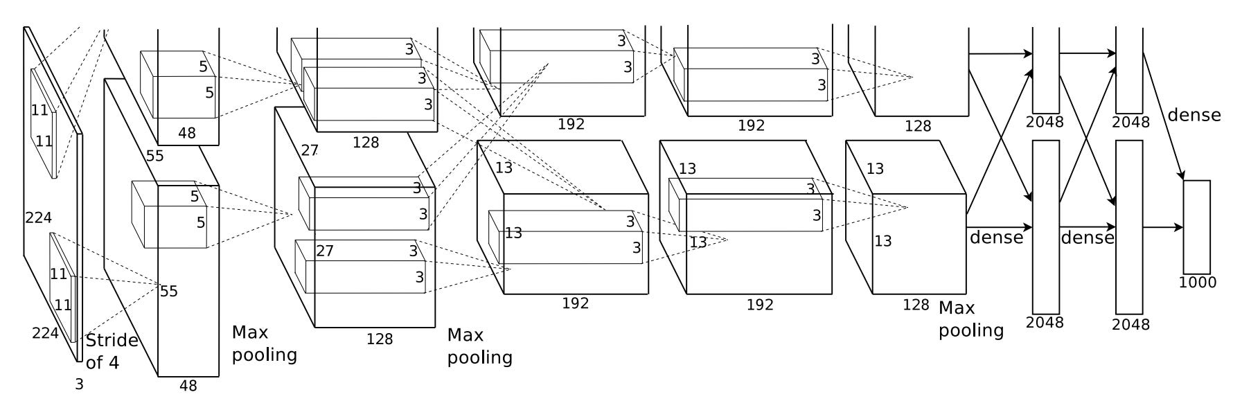
AlexNet trounced the competition at the ImageNet Large-Scale Visual Recognition Challenge (ILSVRC), ushering a high-capacity, compute-driven era of deep learning.
It would be followed by a variety of improvements that have since become commonplace, most notably residual connections (see ResNet, ResNeXt, SqueezeNet, etc.).
2015: DeepLab: Dilation, Segmentation, and Pretraining
I’m certain DeepLab isn’t the first architecture to leverage all of these ideas individually—it appeared roughly the same time as the ubiquitous U-Net architecture, and semantic segmentation technically precedes it by over a decade—but it provides a handy vessel for touching on all of them at once.
Object classification (labeling images as one of various classes) and detection (putting labeled bounding boxes around objects in images) are cornerstone problems of computer vision.
But typical object classification is fairly coarse: you’re classifying an entire image at once. Detection is better—bounding boxes are localized—but it still leaves something to be desired.
In contrast, segmentation seeks to classify individual pixels. For example, take a look at this image/label overlay from the CityScapes dataset:

Semantic segmentation seeks to classify pixels per class, while instance segmentation aims for the further specificity of labeling individual instances of each class separately.
Although segmentation calls for a higher precision than classification or recognition, it seems reasonable that many of the features used in classification of everyday objects should be helpful (at least to start) when trying to segment them. Why not reuse these “pretrained” model weights? This was the question the authors of DeepLab asked.
There was a problem, of course: classification networks continually downsampled their features into small, dense-layer-friendly volumes, implying commensurately tiny weights. How could they reuse those tiny, info-rich weights while still getting a reasonably sized segmentation output?
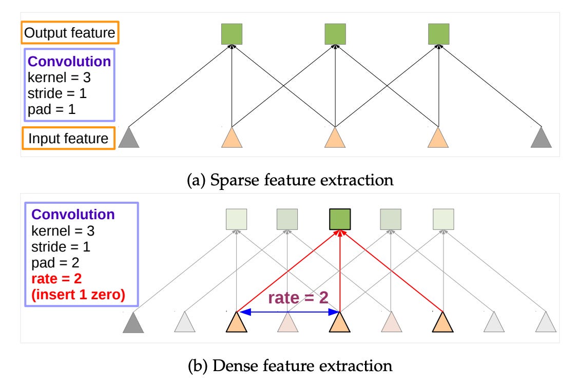
DeepLab’s answer is quite intuitive: in the authors’ words (emphasis added),
remove the downsampling operator from the last few max pooling layers of DCNNs and instead upsample the filters in subsequent convolutional layers, resulting in feature maps computed at a higher sampling rate (1).
In other words, simply stop downsampling your feature volume, and “blow up” the weights (with what’s called a dilated convolution) to match the new, larger size. The benefit: convolution using the smaller weights, but with same-size output—no downsampling! (You can also used dilated convs to yield larger outputs.)
To make a DeepLab segmentation backbone, take your favorite classification CNN, remove the last few downsamples, dilate the last few convolutions, and tack on a classification module at the end (optional: make it learn quicker than the rest, since it’s starting from scratch).
This is trivial to implement for many modern architectures—the ResNet family, AOGNets, etc—and it lower-bounds how small your features get (typically, each swap to dilation will prevent a 2x reduction in resolution), while still enabling the use of those sweet, sweet pretrained weights.
With DeepLab, DLers could leverage weights that were pretrained on classification, without ending up with the tiny output volume of a classification network: it enabled “recycling” the learned features of ImageNet classification (at that point a popular challenge) for semantic segmentation of other datasets.
As it turns out, this is often a good idea. If you don’t believe me, try it yourself: train a DeepLab segmentation network from scratch on CityScapes, and then with ImageNet pretraining. The difference should be severe. Or, take someone else’s word for it:
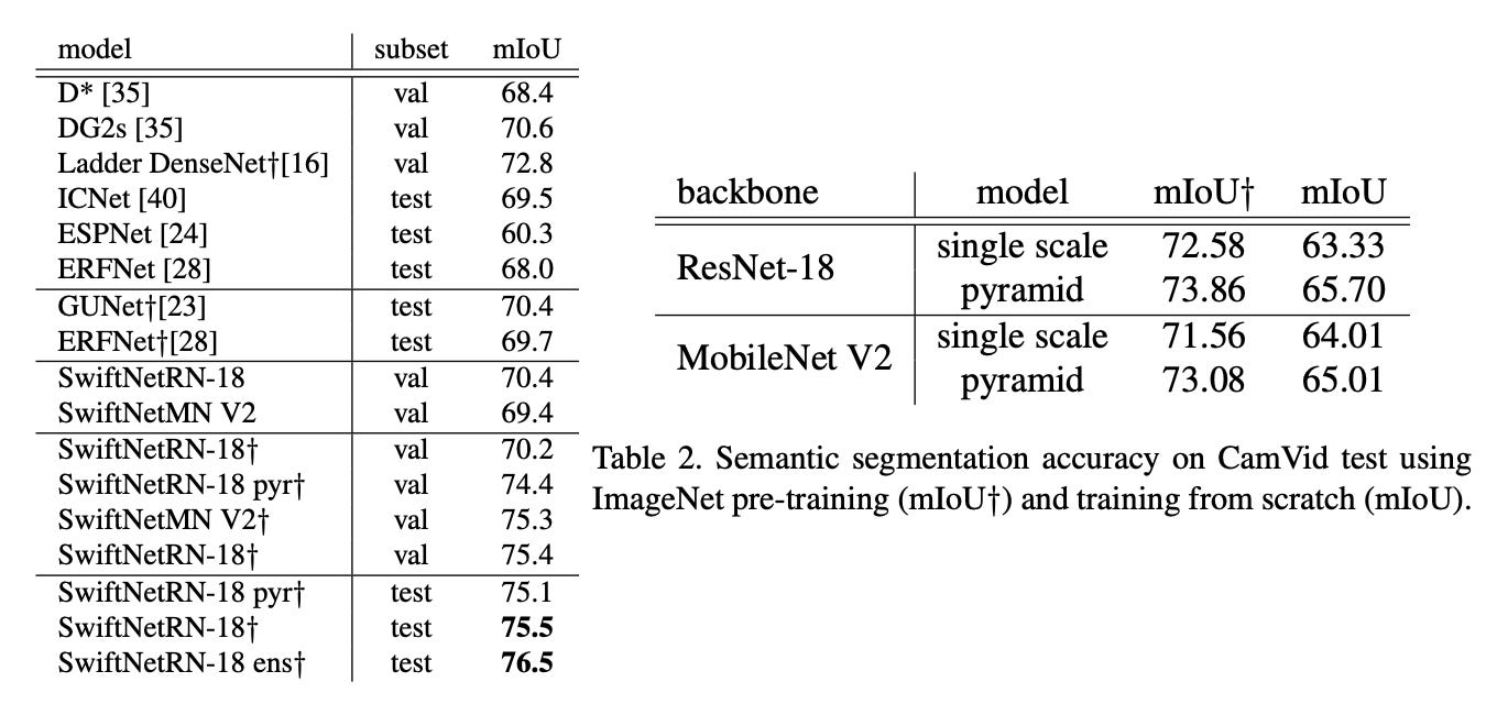
The year it debuted, DeepLab held the highest score yet on CityScapes segmentation (per Papers with Code).
2017/2018: Capsule Networks
Capsule networks improved upon the standard CNN by incorporating more insights from human vision. Two versions appeared, by the same authors, in quick succession: Capsules and Matrix Capsules. I’ll blend together the key features.
(You might think: why are capsule networks more important than residuals? My answer: (1) they are more distinct in motivation; and (2) if you’re sufficiently informed to have this opinion, you may have reached the point of diminishing returns in this review.)
The motivation behind capsule networks goes something like this:
A viewpoint change is a complex, nonlinear transformation of image pixel intensities, but
A viewpoint change is a simple, linear change of an object/viewer pose matrix.
In short, capsule networks try to explicitly model the viewpoint variation that traditional CNNs simple try to ignore (through pooling). While a convolution outputs a scalar, a capsule outputs a vector, and a matrix capsule outputs a (pose) matrix. There’s a nice separation of object instance properties (the direction of the vector / values of the matrix) from object probability (the magnitude of the vector / agreement between matrices).
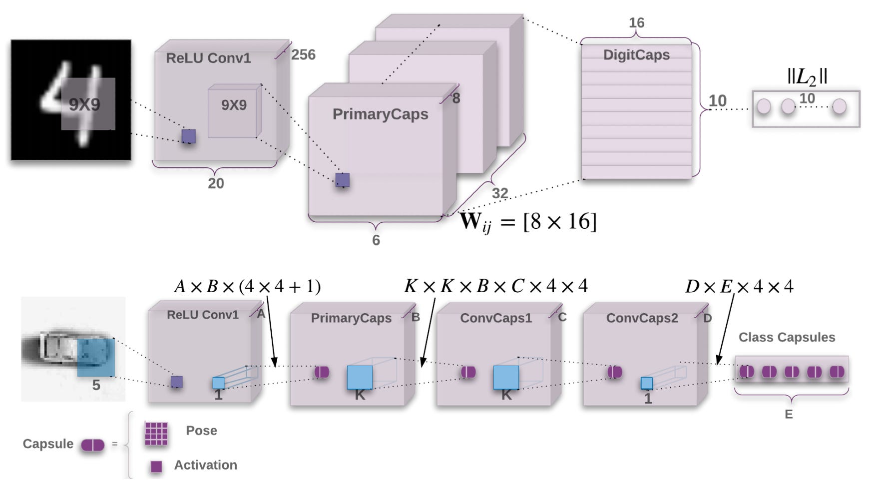
Capsule Networks accomplish object recognition through agreement between “votes” for its pose matrix, which come from object-part capsules, and so on—capsules in one layer have to decide which sort of object (or higher-level “part”) their current “part” belongs to. This process is handled by an algorithm called routing by agreement, and, as the authors point out, it is handily viewpoint-invariant:
As the viewpoint changes, the pose matrices of the parts and the whole will change in a coordinated way so that any agreement between votes from different parts will persist (1).
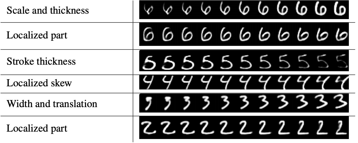
The property-separation of both vanilla and matrix capsules yields a performance boost on viewpoint-variant datasets as well as some nice interpretable property separation. For example, the original Capsule Networks featured a final layer of “Digit Capsules” preceding both classification and input reconstruction; once trained, they seemed to capture interpretable object properties, as shown below.
Capsule Networks haven’t exactly rocketed into ubiquity the way convolutional neural networks did, but in my mind they are almost as fundamental a leap in the field. It’s possible they’re simply hamstrung by computational heft and implementation complexity—keep an eye out for their increased adoption as both of those barriers erode.
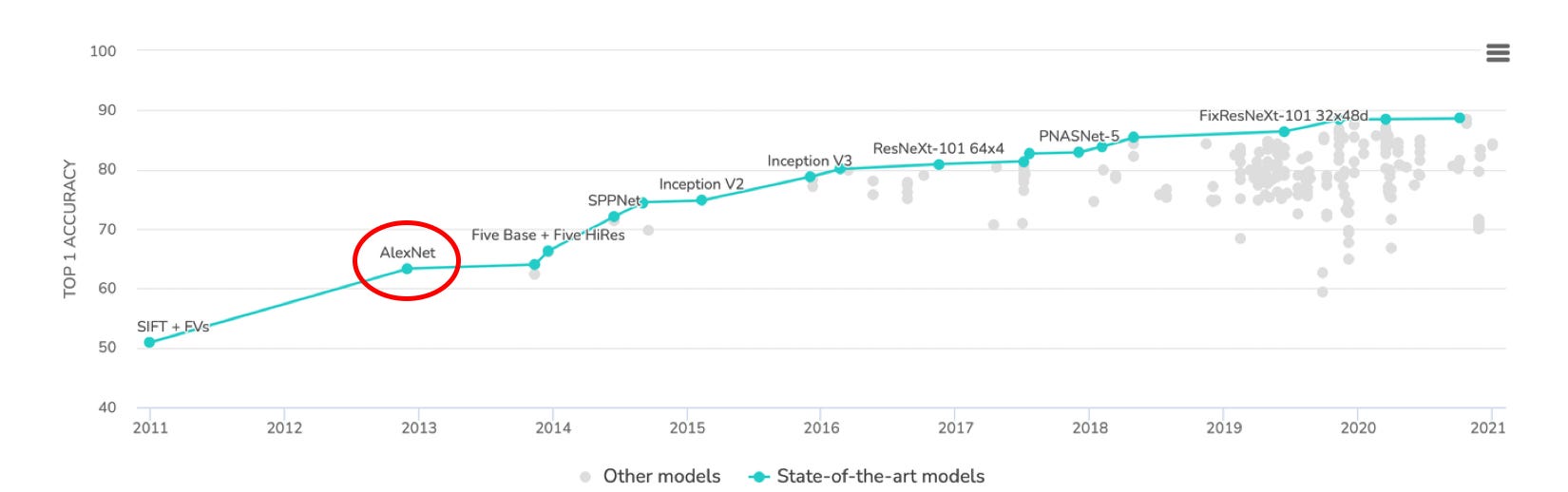
Over time, convolutional architectures have grown more complex, incorporating a variety of architectural improvements motivated by both ML and cognitive theory. AlexNet was revolutionary, but in less than a decade it has grown wholly obsolete. A quick glance at the ImageNet challenge on Papers with Code shows just how far we’ve come:
2020: Transformers Change Lanes
Recently there’s been a surge of interest in transformers, a kind of neural network suited to sequences. Though most of transformers’ breakthroughs have been in natural-language processing—see, for example, GPTs 2 and 3—recently they’ve kicked ass in unconventional fields, including protein folding (at time of writing, the best explanation for AlphaFold 2’s use of them is here).
But perhaps most surprising was their application, this year, to computer vision.
Image-GPT took the transformer architecture and willfully applied it to a domain in which it had no biological motivation. By feeding a transformer architecture images as sequences of RGB pixels, the authors of Image-GPT were able to achieve competitive results in both generative modeling and classification:
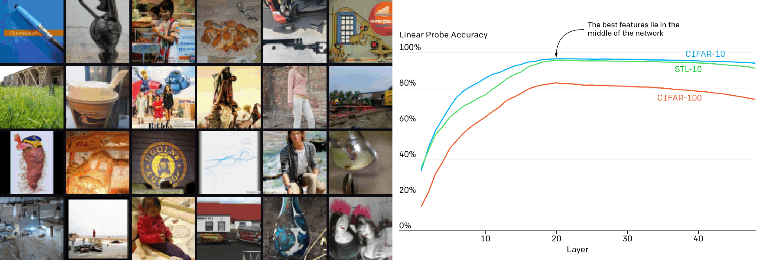
Generative models, as opposed to the discriminative models we’ve covered, attempt to model a data distribution such that new examples may be sampled (or “generated”) from the learned distribution.
There were a few intriguing findings (aside from the generic “oh shit”). First, the authors note that feature quality is an approximately logarithmic function of model depth, suggesting
…that a transformer generative model operates in two phases: in the first phase, each position gathers information from its surrounding context in order to build a contextualized image feature. In the second phase, this contextualized feature is used to solve the conditional next pixel prediction task.
Second, the authors confirmed that generative and discriminative performance were correlated:
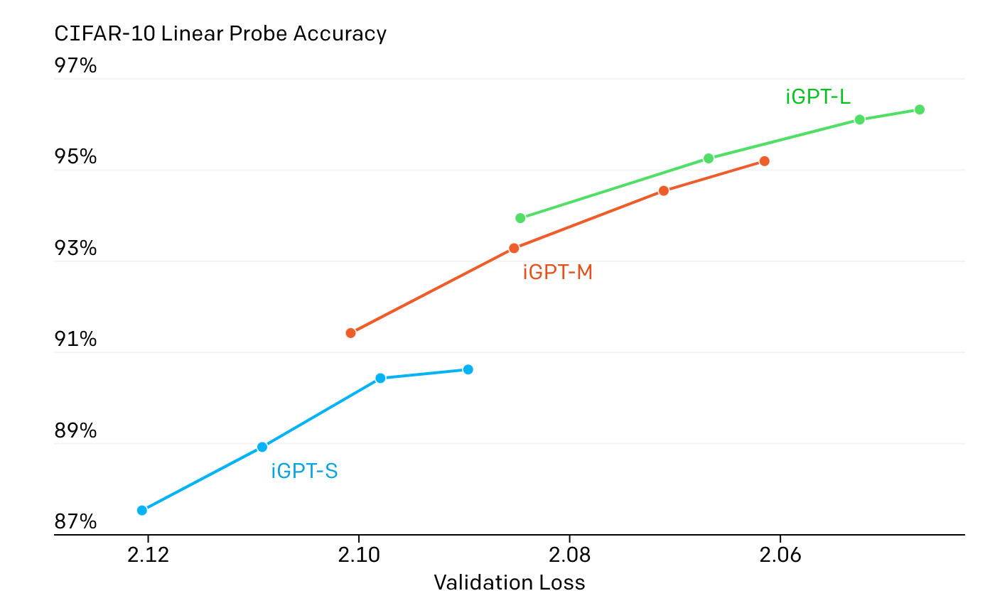
What’s most powerful about the work is how it constitutes a departure from the legacy of convolutional computer vision: there is nothing intuitively “human” about how transformers work in the image domain, and yet they do. And sometimes, when combined with convolutions (as in AlphaFold), they can shatter the state of the art in foreign fields.
I take it as a sign of things to come. Which brings us to the end of our brief history: in the present, looking to the future.